The Basis Trade in a Volatile Regime: Systemic Risk and Market Fragility

Ever since the Federal Reserve started the easing cycle on September 18^th 2024 with a 50 basis point cut, which coincides with the start of the easing cycle in 2007 when the Fed also cut interest rates by 50 bps on September 18^th 2007, there has been a lot of attention and coverage on the US Treasury market both at the front end and at the long end of the curve.

For the front end of curve the 2 year treasury is the one that most investors pay attention to because it is more sensitive to rate hikes or cuts from the FED and some investors on Wall Street, like the bond king Jeffrey Gundlach, even claim that it is the 2 year that dictates the decisions of the FED. As far as the long end of the curve we usually refer to the 10 year treasury which is not only influenced by rates decisions but most importantly by growth and inflation expectations of the market participants.

These two rates have been moving substantially in the last few months after the election of President Trump as more and more uncertainty was priced in by investors; for example as soon as president Trump won the election we saw a significant increase in the 10 year yield as more investors priced in a substantial increase of growth and inflation expectations due to the proposed policies from the white house like less regulation, less red tape and higher tariff to incentivize foreign companies to invest in the USA. After that the 10 year has gotten back down again but generally speaking, what we have seen in the last six months is that the volatility on the bond market has been significant and this is really important because when it comes to bonds, especially government bonds, a move of 40 basis points in a matter of few days is not only uncommon but it has all kinds of implications for the stability of the world financial system that it is still based on the US treasury as the pristine collateral. In today’s white paper we are going to talk about one of the implications of a quick spike of volatility in the bond market which is the unwinding of the Basis Trade.

Our white paper will be divided in three parts: in the first one we will describe how a basis trade works, what are the financial institutions involved and then we will describe the model that we implemented; in the second part we will talk about the risks of this investment strategy and in doing so we will talk about the conditions that can cause this trade to be unwound and in the last part of the paper we will talk about what kind of Facility the FED wants to implement to prevent the Basis trade to be unwound and in doing so we will briefly talk about how the FED’s mandate of financial stability is constantly changing, based on what happens in the financial markets.

The basis trade, in this case the Treasury Cash-Futures Basis Trade, is described in detail in the Federal Reserve notes published in the paper “Quantifying Treasury Cash-Futures Basis Trades” (Barth et al., 2021).

“Is a convergence trade that profits off the spread between the price of Treasury futures contracts and the Treasury securities that can be delivered into those futures”, in other words, this trade exploits the difference in prices between a Treasury security and a related Treasury futures contract – the so-called cash-futures basis – by purchasing the asset that is relatively undervalued and selling the other in a bet that the prices will converge and so ultimately speaking, the trade's profit is based on the difference in the prices paid and received for the cash and futures legs, net of carry and financing costs. The profit of this trade, which consists of a few basis points, as the name suggests requires a lot of leverage to make a meaningful impact on the revenue of the financial institution that is involved.

This profit can be measured in several ways but to stick to the formula used by the FED in their paper, we will consider it in terms of the expected annualized return on a trade that sells a Treasury futures contract and simultaneously purchases the associated cheapest-to-deliver bond, financing the bond in term repo until the optimal futures delivery date. A positive basis indicates that the futures contract is relatively more expensive than the cash security, so that an arbitrageur can expect to profit from a trade that is short a Treasury futures contract and long a Treasury security (referred to as the "long basis trade"). The measure used by the FED considers the optimal delivery timing and bond-specific repo rates, which may result in a different selection of the cheapest-to-deliver bond and that is the option-adjusted basis net of carry (OABNOC), expressed as an annualized yield.

where:

• \(\text{CF}\) represents the futures conversion factor,
• \(\text{PF}\) represents the futures price,
• \(\text{AI}\) represents the accrued interest on the bond,
• \(\text{O}\) represents the estimated value of the options embedded in the futures contract,
• \(\text{PT}\) represents the dirty price (full price) of the cheapest-to-deliver Treasury bond,
• \(\text{R}_\text{repo}\) represents a repo rate quoted by a major broker-dealer for a bond-specific term repo expiring in \(t\) days,
• \(t\) is the number of days until the optimal futures delivery date.

This expression reflects the annualize t days holding period return for the basis trader, accounting for the inflows from the sale of the futures contract, the delivery option value, and the outflows from purchasing the Treasury security and financing it in repo. Optimal delivery of the futures contract in t days, which also corresponds to the assumed holding period of the trade, is determined by whether the position has a positive or negative carry. If the marginal financing cost exceeds the marginal revenue of extending the trade's holding period, we assume that the basis trader will deliver the Treasury security into the futures contract on the earliest date; otherwise, we assume the basis trader delays delivery until the last delivery date.

As we can see in this definition, the basis trade, although very simple in the concept, can involve multiple financial institutions as well as many markets and so it is important to understand, even in simple terms, how a basis trade can be performed by the typical financial firm which is a Hedge Fund. In this strategy the Hedge Fund wants to buy the treasury in the cash market and at the same time it wants to sell the futures on that treasury in order to benefit from the difference between these two prices but it wants to put only a small part of its capital to engage in this trade.

The way the trade will work is that the Hedge fund will go into the Repo market to borrow the money, at the repo rate, which is very short term, to buy the treasury but since repo are collateralized it will use the treasury that it wants to buy as collateral for the loan itself and after buying the treasury in the cash market it will simply go to futures market to sell the futures on that treasury.\\ The idea behind this trade is that the Hedge Fund will have to roll over its repo debt every time it matures since it is very short term and when it has to deliver the treasury that it sold the futures for in the futures market it will use the money received in the futures market to pay back the money borrowed in repo and the difference between what he has borrowed and what he has received for the sale of the futures is its profit and since it is very small it can require a lot of leverage to be substantial for a large financial institution and so Hedge Funds will likely put a small fraction of their capital at risk, which is represented by the haircut of the repo, and borrow a lot of money in the Repo market.

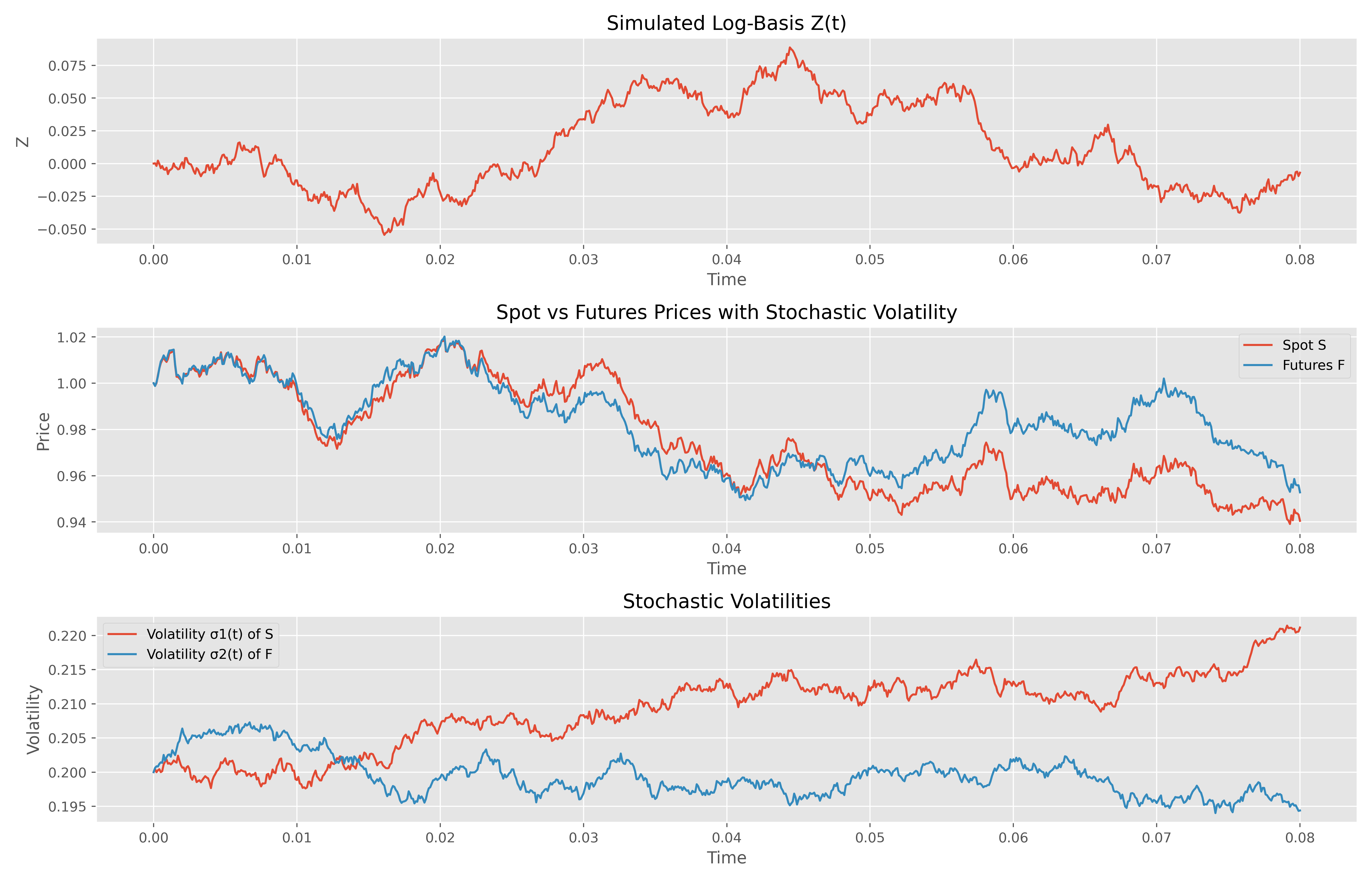
We consider the stochastic basis trading model developed by Angoshtari and Leung (2019), in which a risk-averse investor dynamically allocates wealth between a spot asset \( S_t \) and a futures contract \( F_t \) over a finite trading horizon \([0, T]\). The spot and futures prices follow the volatility-normalized dynamics:

\[ \frac{dS_t}{S_t} = \mu_1 \, dt + dW_{t,1}, \] \[ \frac{dF_t}{F_t} = \left( \mu_2 + \frac{\kappa Z_t}{T - t + \varepsilon} \right) dt + \rho \, dW_{t,1} + \sqrt{1 - \rho^2} \, dW_{t,2}, \]

where \( Z_t = \log(S_t/F_t) \) denotes the log-basis. It evolves according to:

\[ dZ_t = \left( \mu_1 - \mu_2 - \frac{\kappa Z_t}{T - t + \varepsilon} \right) dt + (1 - \rho) \, dW_{t,1} - \sqrt{1 - \rho^2} \, dW_{t,2}. \]

The investor controls the (volatility-adjusted) positions \( \pi_{t,1} \) in \( S_t \) and \( \pi_{t,2} \) in \( F_t \). The associated wealth process \( X_t \) satisfies:

\[ dX_t = \pi_{t,1} \frac{dS_t}{S_t} + \pi_{t,2} \frac{dF_t}{F_t}, \] \[ = \left( \mu_1 \pi_{t,1} + \left( \mu_2 + \frac{\kappa Z_t}{T - t + \varepsilon} \right) \pi_{t,2} \right) dt + (\pi_{t,1} + \rho \pi_{t,2}) \, dW_{t,1} + \pi_{t,2} \sqrt{1 - \rho^2} \, dW_{t,2}. \]

The authors address the problem of optimal trading by considering a utility maximization objective:

\[ \sup_{\pi \in \mathcal{A}} \mathbb{E}_{t,x,z}[U(X_T)], \] where \( U \) is a HARA (Hyperbolic Absolute Risk Aversion) utility function, which includes power (CRRA) and exponential (CARA) forms. The admissible strategies \( \pi \) are subject to the dynamics of the wealth process \( X_t \) and the log-basis \( Z_t \).

They formulate the problem as a stochastic control problem and solve it using dynamic programming techniques. This leads to a Hamilton-Jacobi-Bellman (HJB) equation for the value function \( V(t, x, z) \), which they reduce by assuming a separable ansatz:

\[ V(t, x, z) = U(x) \exp(f(t) + g(t) z + \tfrac{1}{2} h(t) z^2), \] where the functions \( f(t) \), \( g(t) \), and \( h(t) \) satisfy a system of coupled ordinary differential equations. In particular, \( h(t) \) solves a nonlinear Riccati equation whose solvability depends on the investor's risk aversion and the time horizon.

Using this approach, they derive a closed-form expression for the optimal strategy \( \pi^* \) by maximizing the HJB integrand with respect to the controls. The resulting expression is:

\[ \pi^*(t, x, z) = \begin{pmatrix} \pi^*_1(t, x, z) \\ \pi^*_2(t, x, z) \end{pmatrix} = \delta(x) \left[ \begin{pmatrix} \frac{\mu_1 - \rho \mu_2}{1 - \rho^2} + g(t) \\ \frac{\mu_2 - \rho \mu_1}{1 - \rho^2} - g(t) \end{pmatrix} + z \begin{pmatrix} h(t) - \frac{\kappa \rho}{1 - \rho^2} \\ - h(t) + \frac{\kappa}{1 - \rho^2} \end{pmatrix} \right], \]

where \( \delta(x) \) is the investor's risk tolerance function, and \( g(t) \), \( h(t) \) are time-dependent functions determined by the HJB system.

The optimal strategy \( \pi^*(t, x, z) \) is expressed in terms of volatility-normalized positions. That is, instead of specifying the dollar amounts invested in the spot and futures assets, the strategy reflects the exposures scaled by the respective asset volatilities. This normalization simplifies the analysis by setting the diffusion coefficients of the asset price processes to unit volatility, as in the definitions of \( S_t \) and \( F_t \).

To recover the actual dollar positions \( \tilde{\pi}_{t,i} \), one divides the volatility-adjusted positions \( \pi^*_{t,i} \) by the instantaneous volatility \( \sigma_{t,i} \) of each asset:

\[ \tilde{\pi}_{t,i} = \frac{\pi^*_{t,i}}{\sigma_{t,i}}, \quad i = 1,2. \]

This distinction is critical in implementing the strategy empirically, where the raw (unscaled) asset prices are observed.

Volatility-Normalized Strategy Interpretation

The optimal strategy \( \pi^*(t, x, z) \) is expressed in terms of volatility-normalized positions. This means that the strategy prescribes the amount of exposure in terms of units of risk rather than raw dollar amounts. Specifically, the underlying asset prices have been transformed so that their volatilities are equal to one. This simplification allows the investor's optimization problem to avoid explicitly tracking time-varying volatility terms.

To recover the dollar value of the positions in practice, the investor must rescale the normalized strategy by the actual instantaneous volatilities of the assets:

\[ \tilde{\pi}_{t,i} = \frac{\pi^*_{t,i}}{\sigma_{t,i}}, \quad i = 1,2, \]

where \( \sigma_{t,i} \) is the true volatility of asset \( i \). These rescaled quantities \( \tilde{\pi}_{t,i} \) represent the actual investment levels in dollar terms.

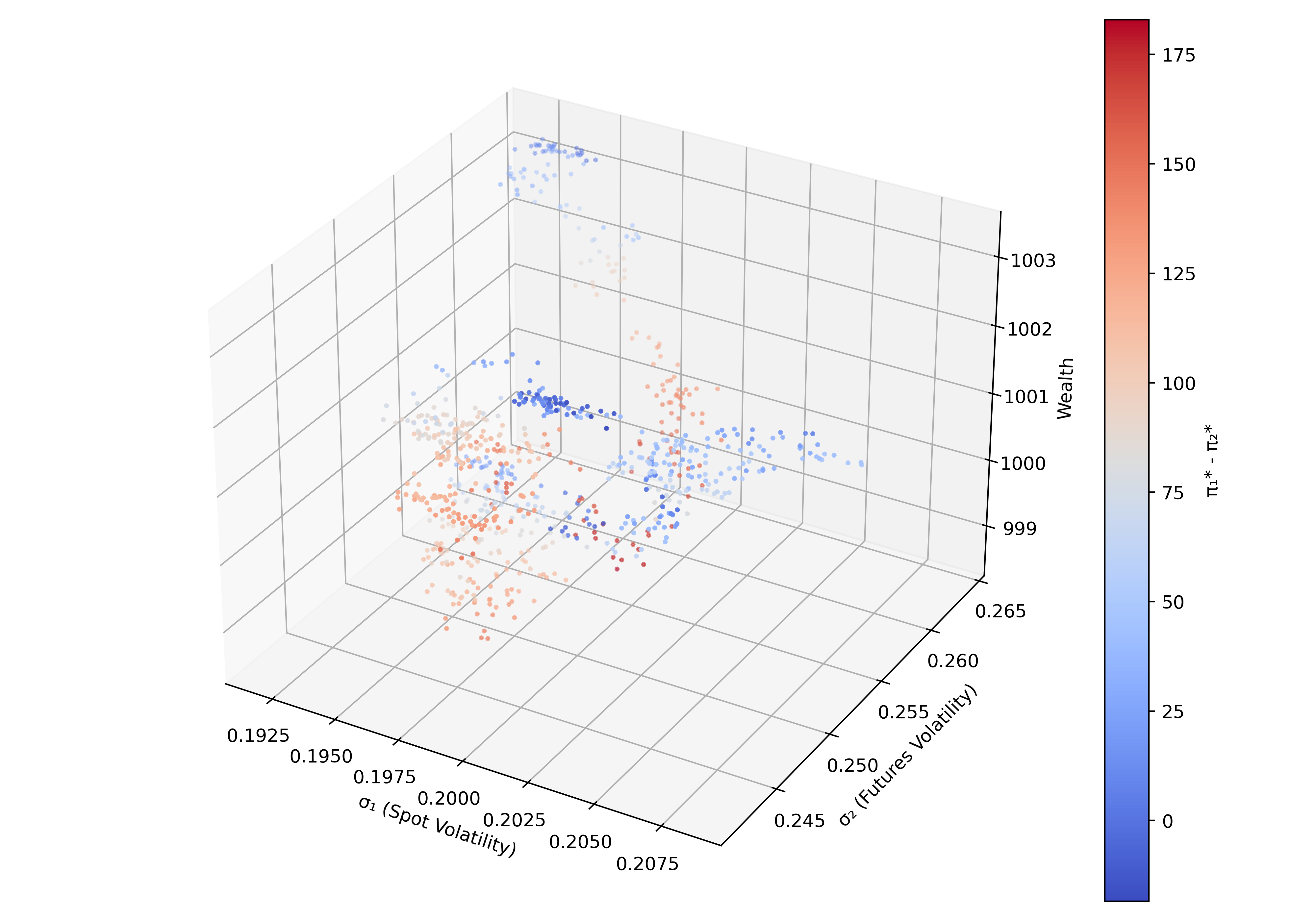
Extension to Stochastic Volatility

Suppose that the volatilities of both the spot and futures prices follow stochastic differential equations. Specifically, let \( \sigma_{1,t} \) and \( \sigma_{2,t} \) denote the instantaneous volatilities of the spot and futures prices, respectively, and assume they evolve as mean-reverting diffusion processes:

\[ \begin{aligned} d\sigma_{1,t} &= \alpha_1(\theta_1 - \sigma_{1,t})\,dt + \eta_1\,dB_{t}^{(1)}, \\ d\sigma_{2,t} &= \alpha_2(\theta_2 - \sigma_{2,t})\,dt + \eta_2\,dB_{t}^{(2)}, \end{aligned} \]

where \( \alpha_i > 0 \) is the speed of mean reversion, \( \theta_i > 0 \) is the long-run average volatility, \( \eta_i > 0 \) is the volatility of volatility, and \( B_t^{(i)} \) are Brownian motions, possibly correlated with each other and with the Brownian motions driving asset prices.

Under this framework, the volatility-normalized prices \( S_t \) and \( F_t \) are defined by scaling the actual (quoted) prices \( \tilde{S}_t \) and \( \tilde{F}_t \):

\[ S_t = \frac{\tilde{S}_t}{\sigma_{1,t}}, \qquad F_t = \frac{\tilde{F}_t}{\sigma_{2,t}}. \]

This transformation ensures unit volatility for modeling purposes but introduces time- and path-dependence due to the stochastic nature of \( \sigma_{1,t} \) and \( \sigma_{2,t} \).

The optimal strategy \( \pi^*(t, x, z) \) remains valid in normalized units, representing positions in terms of risk exposures. To obtain the actual investment levels in dollars, one must rescale the normalized positions using the current values of the volatilities:

\[ \tilde{\pi}_{t,1} = \frac{\pi^*_{t,1}}{\sigma_{1,t}}, \qquad \tilde{\pi}_{t,2} = \frac{\pi^*_{t,2}}{\sigma_{2,t}}. \]

Because \( \sigma_{1,t} \) and \( \sigma_{2,t} \) evolve stochastically, the dollar allocations \( \tilde{\pi}_{t,1} \) and \( \tilde{\pi}_{t,2} \) fluctuate dynamically, even if the normalized strategy \( \pi^* \) is held constant. This implies that the investor must continuously monitor and adjust their actual holdings in response to changes in the volatility environment.

In the stochastic basis trading model, asset prices are normalized by their stochastic volatility to simplify the mathematical formulation. Specifically, the normalized spot and futures prices are defined as:

\[ S_t := \frac{\tilde{S}_t}{\sigma_{1,t}}, \quad F_t := \frac{\tilde{F}_t}{\sigma_{2,t}}, \]

where \( \tilde{S}_t \), \( \tilde{F}_t \) denote the actual (market) prices, and \( \sigma_{1,t} \), \( \sigma_{2,t} \) are their instantaneous volatilities. This transformation ensures that the normalized prices have unit volatility, which facilitates tractable optimization and simplifies the Hamilton-Jacobi-Bellman (HJB) equation governing optimal investment.

Volatility-Adjusted Strategy

The strategy variables \( \pi_{1,t} \) and \( \pi_{2,t} \) denote the investor’s positions in the normalized assets, and are referred to as volatility-adjusted positions. These are expressed in terms of risk exposure per unit of wealth, and they govern the stochastic differential equation for wealth:

\[ dX_t = \pi_{1,t} \frac{dS_t}{S_t} + \pi_{2,t} \frac{dF_t}{F_t}. \]

Conversion to Dollar Positions

To implement the strategy in real financial markets, the volatility-adjusted positions must be converted into dollar amounts. The corresponding dollar positions are:

\[ \tilde{\pi}_{1,t} := \frac{\pi_{1,t}}{\sigma_{1,t}}, \quad \tilde{\pi}_{2,t} := \frac{\pi_{2,t}}{\sigma_{2,t}}. \]

These represent the dollar amount invested in the spot and futures assets per unit of wealth. The actual dollar allocations at time \( t \), given current wealth \( X_t \), are:

\[ \text{Invested in spot:} \quad X_t \cdot \tilde{\pi}_{1,t}, \qquad \text{Invested in futures:} \quad X_t \cdot \tilde{\pi}_{2,t}. \]

Numerical Example

Suppose that at a given time \( t \), the investor has wealth \( X_t = 1000 \), and the volatility-adjusted strategy is:

\[ \pi_{1,t} = 0.3, \quad \pi_{2,t} = -0.2, \quad \sigma_{1,t} = 0.15, \quad \sigma_{2,t} = 0.25. \]

Then the dollar-normalized positions are:

\[ \tilde{\pi}_{1,t} = \frac{0.3}{0.15} = 2.0, \qquad \tilde{\pi}_{2,t} = \frac{-0.2}{0.25} = -0.8. \]

This implies the investor is:

• Long $2000 in the spot asset: \( 1000 \cdot 2.0 = 2000 \)
• Short $800 in the futures: \( 1000 \cdot (-0.8) = -800 \)

Note that the strategy is leveraged: the total gross exposure is $2800, even though wealth is $1000.

Interpretation

The volatility-adjusted strategy \( \pi_t \) is used in the normalized model to derive optimal controls, but actual trading is carried out using \( \tilde{\pi}_t \). This distinction ensures mathematical tractability without sacrificing practical relevance. Notably, dollar positions can exceed wealth (i.e., be leveraged) or be negative (short positions), depending on the sign and magnitude of \( \tilde{\pi}_{i,t} \).

As we saw in the definition of this trade and in the practical example, this simple trade involves several financial institutions that interact with each other in several markets and so the risks of this trade can come from multiple sources.

As we said before, the Hedge fund has to roll over its repo loan anytime it matures and generally speaking, REPO contracts are very short term, even overnight instruments so if repo rates spike because, for example, the perceived counterparty risk rises significantly, like in September 2019, then the Hedge fund will have to borrow a lot more money to roll over its debt and if the repo rates rises to a certain point, then the Hedge Fund will simply not get enough money from the sale of the futures to pay back its debt and so what will likely happen is that the repo counterparty will take the treasury away from the Hedge Fund and since this trade is on very high levels of leverage, it can mean substantial losses for the financial firm that sold the futures as well as the one who bought the futures contract.

Another risk comes from the Futures market and so what could happen is that if interest rates on treasury go up significantly in a very short time period, which is what we have seen in March 2020 and in at the beginning of April, then the value of the treasuries involved in the futures contract will go down and so the clearing house that acts between the seller of the futures and the buyer of the futures will issue a margin call to make the seller put additional capital to offset the losses and if the hedge fund does not do that, then the clearing house will take away the futures contract from the Hedge Fund and give it to a lesser risky counterparty since the clearing house has not legal right to take the treasury as it was put as collateral in the repo market and ultimately the Hedge Fund will lose its margin for the futures contract.

The quick rise in interest rates can also impact the Repo Market because if interest rates rise substantially, then the Hedge Fund will need to put additional capital to offset the loss of value of the treasury used as collateral in the repo market and if it does not, then it will need to sell the treasury to pay back the loan but this will represent a loss for the repo market dealer because it lent more than what it is able to get back from selling the treasury, especially if we are talking about a “Off the run” treasury and so liquidity in the repo market will likely contract and that could put upward pressure on repo rates which could cause all kinds of problems for the stability of the global financial system.

In this white paper we have seen how a quick spike of volatility in the Treasury Market can cause all kinds of problems for the several financial institutions that deal with each other in the markets and that is partially why the FED has paid a lot of attention to the “Financial Stability” aspect of its mandates and so whenever we had some problems in the US treasury market, the FED immediately set up a Facility to prevent a distressed sale of treasuries pushing interest rates even higher.

As an example, during the Covid 19 crisis, the FED acted quickly by setting up Swap Lines and the FIMA facility to help foreign central banks to deal with the dollar shortage that they were facing and so instead of selling these treasuries in a troubled market, they could repo these treasuries directly with the FED. During the banking crisis of march 2023 the FED set up a new facility for banks, the BTFP program, to prevent them from selling US treasuries that had lost so much value due to the rate hikes; in doing so the FED was able to purchase these bonds at par to prevent the banks to incur in any losses and so they were able to pay their depositors back.

As far the basis trade, the Federal Reserve is paying close attention to it because it recognize its magnitude and its importance for the correct functioning of the futures markets and the Repo market and that’s why it is thinking about setting up a new facility for a small group of Hedge Funds to bail them out in case of any trouble in the US treasury market with the same goal of preventing them to fire-sale these treasuries in a panic situations causing the long end of the curve to go really high resulting in all kinds of problems for the stability of the global financial system.

References

Bahman Angoshtari and Tim Leung. Optimal Dynamic Basis Trading, 2019.
Available at:
https://arxiv.org/abs/1809.05961
Daniel Barth, R. Jay Kahn, et al. Hedge Funds and the Treasury Cash-Futures Disconnect.
OFR Working Paper 21–01, 2020.