The Bond Vigilantes and their impact on the 10 Years US Treasury
Table of Contents
Introduction
When it comes to trading and investing, fixed income instruments constitute an important asset class for every portfolio so it is important to understand what are the drivers for the yield of these instruments. Governments around the world issue bonds to finance their deficits and to rollover their debts so the bond market is one of the largest and most important market in the world.
Within all bond markets, the US Treasury Market is the most liquid and sophisticated one and that is because of the dollar’s role as the global reserve currency. Due to the importance of the dollar as the cornerstone of the financial system, US treasuries are held all around the world by public and private institutions and these instruments are used as collateral for almost all the financial transactions that take place in the global markets as the US treasury is considered the benchmark instrument for the so called risk free return.
The US Treasury Market, like many other bond markets, is very vast and there are instruments with different maturities but in this white paper we are going to focus on the 10 Years US Treasury which is considered the pristine collateral of the global financial system and so we will try to understand what are the most important drivers of this security’s yield.
This paper is organized into six main sections. Following the Introduction, Section 2 presents the Supply Argument, exploring the traditional view that rising government debt should increase Treasury yields, and assesses the sustainability of debt using the Debt-to-GDP ratio. Section 3 introduces the Bond Vigilantes phenomenon, which refers to investors who may enforce fiscal discipline by selling government bonds when they perceive fiscal or monetary irresponsibility. Section 4 presents the Demand Argument, showing that the 10-year yield appears to track expectations about inflation and economic growth more closely than fiscal metrics. Section 5 applies Principal Component Analysis and a Markov-switching framework to identify distinct regimes in yield dynamics and interprets them in terms of macroeconomic drivers related to bond vigilante behavior. Section 6 concludes with Final Considerations, comparing the PCA-based and macro-core models, discussing their respective strengths and limitations, and evaluating the overall robustness of the bond vigilante framework.
The Supply Argument
There is too much debt, the US will default, the FED will have to monetize the Debt and implement Yield curve control
We all understand that the yield of any security is influenced by so many variables that analyzing every single one simultaneously is basically impossible so what we are going to do, as economists, is working on the variables that we want to study and in doing so we will assume that the others stay the same “Ceteris Paribus” to isolate the effect of the ones that we are considering.
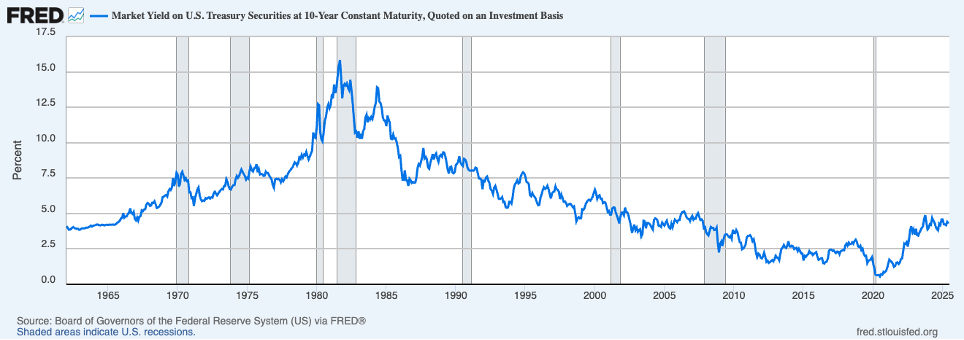
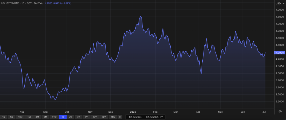
This chart represents the yield of the 10 Years US treasury, and as we can see, the yield peaked in September 1981 at 15.84%, then it went down dramatically to reach a new high in may 1984 when it got to 13.91%, approximately 200 bps lower than the previous high. After these two peaks, the yield went down dramatically during the great moderation and in the early 2000s. And now it is currently trading around 4.3%.
The yield has been trending lower and so, if we assume that the demand has remained the same, then the supply of it would have had to drop so that the price would have gone up pushing the yield down... Since we are talking about a debt instrument, the supply is represented by the amount of debt that is issued by the government and so we need to look at the amount of debt issued by the US government.
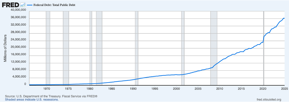
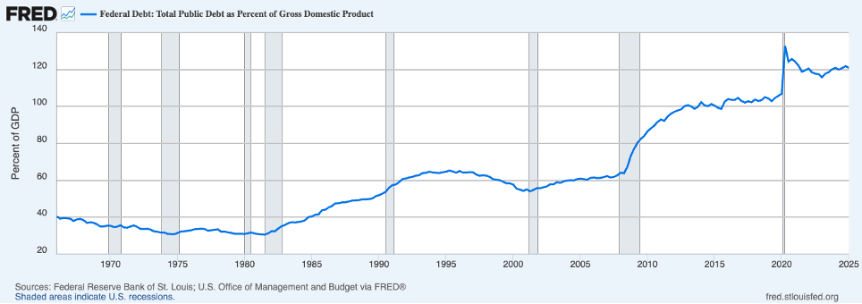
As we can see in this chart, the US debt increased significantly from the 1960’s to nowadays so the supply of treas uries went up dramatically and yet the yield went down. Now, to be fair we have to point out the fact that the US government finances itself with fixed income instruments of almost every maturity but still, the supply of the 10 Years US Treasury has certainly gone up but the yield has gone down so we need to investigate further. Having said that, someone could argue that is not the supply of treasuries that is relevant per say but its sustainability that counts and that is represented by the Debt/GDP ratio because if you have an economy where GDP grows faster than its debt, than the debt is sustainable because it can be paid with the growth that the economy is able to generate so let’s see a chart of the Debt/GDP ratio to see if something changes.
The Bond Vigilantes
As we have seen in these charts, as the fiscal situation of the US has gotten worse, the yield on the 10 Years US Treasury has declined significantly from the 1980’s peak so someone could argue: why should we assume that as more US treasuries are issued, the yield of them will go up? Behind the simple fact that as more US treasuries are issued, the supply of them will go up and so if we assume that the demand stays the same, then the price will have to fall putting upward pressure on the yield; there is also another phenomenon that is usually used in finance to describe a situation where the government needs to keep its fiscal house in order otherwise it will pay with higher long term yields and it is called “The bond vigilantes phenomenon” but let’s see what it is about. The bond vigilantes are fixed income investors that hold a significant amount of government bonds of a country, especially the long end of the curve, and what they will do is watching very closely the fiscal and monetary policies of a country and if they think that the government, or the central bank is acting irresponsibly, they will sell their treasuries into the market to push long term yields up and to prevent this bad policies from happening. As an example, let’s say that a country has a very high Debt/GDP ratio and is facing high inflation, then if its government proposes to pass a big deficit to stimulate the economy, then the vigilantes, will sell a significant amount of treasuries into the market to push long term rates up making it harder for the government to finance its debt and in that situation the government will likely back down from its intentions causing long term yield to go back down again.
Now let’s see if the bond vigilantes are showing up in the US treasury market and so we will look at the spread between the FED funds rate, that is controlled by the FED, and the 10 Years US treasury and if they are actually there, maybe because the US Governments is likely to pass “The big beautiful bill” or because the president is introducing a lot of volatility in the market with these tariffs announcement or simply because the USA just got downgraded by another rating agency, then the spread will be high because these vigilantes are dumping treasuries into the market to force some fiscal discipline to the US government.
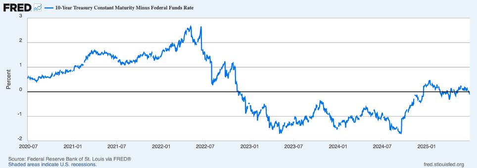
As we can see in this chart, the spread between the 10 years and FED funds is currently negative so that means that short term rates are actually higher than long term rates. Obviously this situation contradicts entirely the bond vigilantes narrative because if they were there selling treasuries, we would see a significant positive spread, instead what we can understand by looking at this chart is that now the demand for the long end of the curve is so high, despite all the fiscal difficulties of the US government, that the yield is lower than Fed funds, which is an overnight rate. Having said that, maybe there is something else that really drives the long end of the curve and that is what we will look at in the next section of this paper.
The Demand Argument
The 10 Years US Treasury seems to track Growth and Inflation expectations.
As we have seen in the last part, the yield on a 10 Years US Treasury has been trending down from the 1980’s peak to nowadays regardless of what has happened with the US fiscal situation but if we put a chart of the 10 year yield and US nominal GDP we see a different picture:
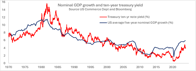
As we can see in this chart, the 10 Years US treasury seems to track well US nominal GDP but if we think about it, what constitutes nominal GDP is inflation and growth and so the idea is that as yield on the long end move, investors expect different levels of growth and inflation. According to this view, the 10 Years US Treasury reflects growth and inflation expectations but let’s try to understand why that might be the case. First of all, let’s think about what low long term rates actually mean because, after all, if these rates are low, that means that demand for safety and liquidity is very high and what is the kind of economy under which these conditions will hold? Certainly not in an economy that is growing substantially because in that case, investors will want to lend in the real economy to fund capital investments and business expansions and in that situation the demand for the safest and most liquid instrument will likely go down, pushing the yield up. Instead, in an economy that is struggling to grow, investor will want to put their money in something that is safe and liquid because, for them, the perceived counterparty risk is too high and so the risk adjusted return is not enough for them.
This view of long term rates can be counterintuitive because it implies that low long term rates are not a symbol of economic strength and loose money, instead the complete opposite because low long term rates represent a high demand for safety and liquidity, so a high perceived counterparty risk and by extension tight money because financial institutions will not lend as loosely as before. This idea, strangely as it sounds, is coherent with the Interest rate fallacy theory explained by Milton Friedman that states that even though interest rates, set by the central banks, might be low, for some borrowers it will still be hard to get credit and so for them, money is tight, not loose. Having said that, long term rates seem to track growth and inflation expectations and so the yield on a 10 Years US Treasury will reflect, at any moment, what investors expect for the future rate of growth and inflation but these expectations can change dramatically, based on what happens in the US economy and in the world’s economy, and that partially explains the volatility that we have seen in this markets in the last year or so.
Principal Component Analysis and Its Relevance for Regime Switching
Principal Component Analysis (PCA) is a statistical technique designed to reduce the dimensionality of a dataset by constructing new, orthogonal variables (called principal components) that successively capture the largest possible variance present in the original variables. Each principal component is a linear combination of the standardized original series, chosen so that PC1 explains the greatest share of total variance, PC2 the next greatest (subject to orthogonality with PC1), and so on. By transforming a high-dimensional macroeconomic panel into a small number of uncorrelated factors, PCA mitigates multicollinearity, filters idiosyncratic noise, and concentrates the common signals driving yield dynamics.
In the context of Markov-switching models for the 10-year Treasury yield, using PCA makes particular sense for two reasons. First, the sheer number of candidate predictors (ranging from inflation expectations and fiscal ratios to real activity and central bank balance-sheet measures) would render a fully parameterized regime-switching model both unwieldy and prone to overfitting. Second, the regimes themselves are hypothesized to reflect shifts in underlying macro-financial conditions (for example, "inflationary pressure" versus "flight to quality"), which are better captured by a handful of latent factors than by individual observable series. By incorporating the first three PCs as regime-dependent regressors, we parsimoniously summarize broad inflation or fiscal dynamics, real-economic stress, and unconventional monetary policy shocks, while retaining the flexibility to allow their effects to vary across high- and low-volatility states.
Interpretation of Principal Components with a Bond-Vigilante Lens
In our analysis, bond vigilantes (investors who sell government bonds in response to perceived fiscal imprudence) play a central role in driving yield dynamics. The first two principal components (PCs) capture the conditions under which vigilante pressure intensifies and pushes the 10-year yield higher.
PC1: Inflationary Macro-Fiscal Pressure
PC1 loads heavily on long-run inflation expectations (T10YIE, T5YIFR), debt-to-GDP, outlays-to-GDP, and the Fed's balance sheet (WALCL). A surge in PC1 reflects a market view of rising inflation combined with aggressive fiscal expansion (exactly the scenario that triggers bond-vigilante selling). As PC1 increases, vigilantes demand higher term premia to compensate for anticipated debt issuance and maturing QE support, thereby raising yields.
PC2: Real-Economy Weakness amid Fiscal Strain
PC2 carries a positive weight on unemployment (UNRATE) and negative weights on industrial production and the deficit-to-GDP ratio. High PC2 signals a sluggish economy coexisting with worsening deficits (a red flag for vigilantes concerned that weak growth will undermine fiscal sustainability). In such episodes, bond vigilantes preemptively sell, forcing yields upward even if inflation pressures are muted.
Implications for Regime Dynamics
In the Markov-switching framework, spikes in PC1 most often precipitate transitions into the high-yield "vigilante scare" regime (Regime 1), where bond vigilantes collectively drive yields sharply higher. Conversely, periods dominated by QE shocks (captured in PC3) can temporarily suppress vigilante influence, anchoring yields in the low-volatility "flight-to-quality" regime (Regime 2). Thus, PC1 and PC2 serve as early warning indicators of bond-vigilante episodes that elevate long-term interest rates.
Comments and Analysis
In Regime 1, despite the slope on PC1 (0.3172) being lower than in Regime 2 (0.5955), the intercept of 3.1996 (substantially higher than Regime 2's 2.6566) creates a uniformly elevated yield baseline, reflecting the market's vigilant stance. Moreover, the negative loading on PC2 (-0.2992) implies that improvements in real activity actually dampen yields only in this regime, consistent with bond vigilantes demanding higher yields predominantly when inflationary and fiscal pressures (PC1) dominate and real growth fails to offset them. Thus, Regime 1 encapsulates periods of heightened market discipline, where yields remain high in spite of PC sensitivities, unlike Regime 2's lower-baseline environment.
| Regime 1 (Bond-Vigilante) | Regime 2 (Flight-to-Quality) | |||
|---|---|---|---|---|
| High-Yield Phase | Low-Yield Phase | |||
| Intercept | 3.1996 | (baseline) | 2.6566 | (lower baseline) |
| PC1 coefficient | 0.3172 | (moderate) | 0.5955 | (strong) |
| PC2 coefficient | -0.2992 | (dampening) | 0.2604 | (reinforcing) |
| Residual SD | 0.9267 | 0.1935 | ||
| R² | 0.4465 | 0.9632 | ||
| To Regime 1 | To Regime 2 | |
|---|---|---|
| From Regime 1 | 0.99586 | 0.00333 |
| From Regime 2 | 0.00414 | 0.99667 |
| Regime 1 (Bond-Vigilante / High-Yield Phase) | ||||
|---|---|---|---|---|
| Estimate | Std. Error | t value | p value | |
| Intercept (S) | 3.1996 | 0.0198 | 161.596 | <2.2×10⁻¹⁶ |
| PC1 (S) | 0.3172 | 0.0096 | 33.042 | <2.2×10⁻¹⁶ |
| PC2 (S) | −0.2992 | 0.0113 | −26.478 | <2.2×10⁻¹⁶ |
| Residual SD | 0.9267 | |||
| Multiple R² | 0.4465 | |||
| Regime 2 (Flight-to-Quality / Low-Yield Phase) | ||||
| Estimate | Std. Error | t value | p value | |
| Intercept (S) | 2.6566 | 0.0040 | 664.150 | <2.2×10⁻¹⁶ |
| PC1 (S) | 0.5955 | 0.0026 | 229.040 | <2.2×10⁻¹⁶ |
| PC2 (S) | 0.2604 | 0.0026 | 100.150 | <2.2×10⁻¹⁶ |
| Residual SD | 0.1935 | |||
| Multiple R² | 0.9632 | |||
| To Regime 1 | To Regime 2 | |
|---|---|---|
| From Regime 1 | 0.99586 | 0.00333 |
| From Regime 2 | 0.00414 | 0.99667 |
Why Regime 1 Captures Bond-Vigilante Episodes
Regimes in a Markov-switching model are defined by the combination of intercept, loadings, and volatility rather than by the largest coefficients alone. In our case:
- Elevated Baseline: Regime 1’s intercept (3.20) far exceeds Regime 2’s (2.66), so even moderate rises in PC1 and PC2 produce uniformly high yields, consistent with bond-vigilante pressure.
- Higher Volatility: The residual standard deviation in Regime 1 (0.93) is much larger than in Regime 2 (0.19), matching the abrupt, jagged yield spikes observed when vigilantes unload bonds.
- Asymmetric PC2 Effect: A negative PC2 loading (–0.30) means that improvements in real activity do not offset inflation/fiscal concerns—exactly the behavior seen when vigilantes remain unconvinced by better growth data.
By contrast, Regime 2 is a low-baseline, low-volatility environment where yields, although more sensitive to PC shocks, stay anchored at lower levels—characteristic of QE-dominated or “flight-to-quality” conditions. Thus, Regime 1 aptly embodies the high-yield, high-variance “vigilante scare” regime.
Full Markov-Switching Model Summary with Bond-Vigilante Commentary
Regime 1:
  GS10_t = 3.1996 + 0.3172 * PC1_t - 0.2992 * PC2_t
  Residual SD = 0.9267, R^2 = 0.4465
This regime exhibits a high intercept and substantial residual volatility, indicating that even moderate fiscal-inflation shocks (PC1) trigger elevated yields. The negative PC2 coefficient shows that real-activity improvements fail to temper yields, consistent with bond vigilantes insisting on higher term premia despite stronger growth.
Regime 2:
  GS10_t = 2.6566 + 0.5955 * PC1_t + 0.2604 * PC2_t
  Residual SD = 0.1935, R^2 = 0.9632
Here, yields respond more sensitively to shocks but are anchored around a lower baseline with minimal volatility, characteristic of QE-dominated or “flight-to-quality” phases where vigilante pressure is subdued.
Transition Probabilities:
  P = [
    [0.99586, 0.00333],
    [0.00414, 0.99667]
  ]
Transitions into Regime 1 occur when PC1 or PC2 spikes surpass vigilante tolerance, while exits are infrequent.
Bond-Vigilante Interpretation
Regime 1 clearly aligns with “vigilante scare” episodes: a high baseline yield, large shocks, and asymmetric real-activity effects mirror episodes where fiscal-inflation concerns prompt aggressive bond-selling. Regime 2, by contrast, embodies periods of policy support and muted vigilante influence.
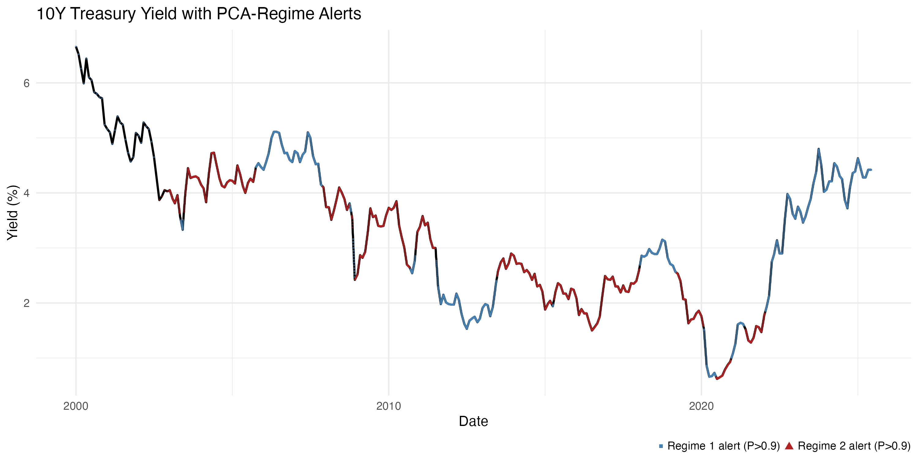
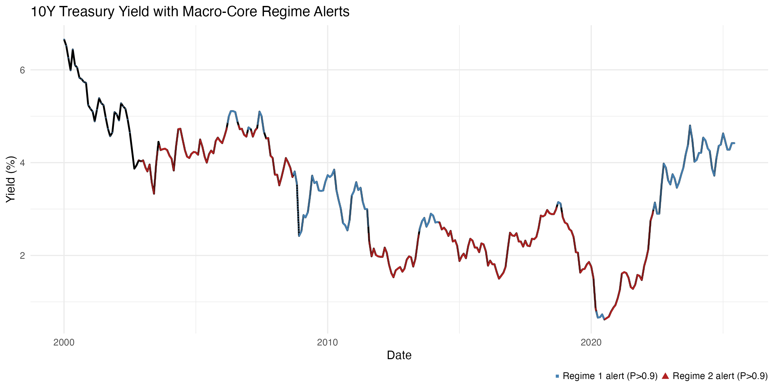
The overlaid markers in Figure highlight periods of high-confidence regime assignment. Steel-blue squares cluster around pronounced yield spikes, indicating episodes when rising PC1 (inflation/fiscal pressure) or PC2 (real-economy weakness) trigger bond-vigilante selling. Firebrick triangles appear during extended low-volatility stretches, consistent with QE-dominated or flight-to-quality phases.
Macro-Core Model Summary
| Regime 1 (Vigilante-Sensitive Phase) | ||||
|---|---|---|---|---|
| Estimate | Std. Error | t value | p value | |
| Intercept (S) | 5.7825 | 0.1035 | 55.870 | <2.2×10⁻¹⁶ |
| T10YIE (S) | 0.6475 | 0.0272 | 23.805 | <2.2×10⁻¹⁶ |
| UNRATE (S) | −0.2166 | 0.0051 | −42.471 | <2.2×10⁻¹⁶ |
| debt_gdp (S) | −0.0022 | 0.0001 | −22.000 | <2.2×10⁻¹⁶ |
| Residual SD | 0.5075 | |||
| Multiple R² | 0.7040 | |||
| Regime 2 (Anchored / Low-Volatility Phase) | ||||
| Estimate | Std. Error | t value | p value | |
| Intercept (S) | 6.5971 | 0.0450 | 146.602 | <2.2×10⁻¹⁶ |
| T10YIE (S) | 0.5906 | 0.0141 | 41.886 | <2.2×10⁻¹⁶ |
| UNRATE (S) | −0.1916 | 0.0035 | −54.743 | <2.2×10⁻¹⁶ |
| debt_gdp (S) | −0.0044 | 0.0000 | — | <2.2×10⁻¹⁶ |
| Residual SD | 0.2611 | |||
| Multiple R² | 0.9474 | |||
| To Regime 1 | To Regime 2 | |
|---|---|---|
| From Regime 1 | 0.99613 | 0.00218 |
| From Regime 2 | 0.00387 | 0.99782 |
Bond-Vigilante Interpretation
Regime 1 exhibits strong sensitivity to inflation expectations (T10YIE) and unemployment, coupled with a higher residual volatility (0.5075), capturing the abrupt yield spikes driven by bond vigilantes reacting to fiscal-inflation signals. In contrast, Regime 2 features lower volatility (0.2611) and somewhat muted parameter responses, reflecting periods where policy support or safe-haven flows anchor yields and suppress vigilante activity.
Final Considerations
Both the PCA-based and macro-core Markov-switching models identify the same high-yield “Regime 1” and low-yield “Regime 2” episodes using a P > 0.9 threshold, and both assign those regimes to periods consistent with the classic “bond-vigilante scare” versus “QE-anchored/flight-to-quality” narrative. Despite differing input specifications, they yield remarkably similar switch dates and economic interpretations:
- PCA-Based Model: Captures broad inflation/fiscal pressure (PC1) and real-economy strain (PC2) as leading drivers of regime shifts. This enhances parsimony and guards against multicollinearity, but obscures which variables drive switches.
- Macro-Core Model: Uses interpretable covariates (breakeven inflation, unemployment, debt-to-GDP), but may overfit or miss latent interactions.
Limitations and Trade-Offs
- Regime Definition: The P > 0.9 threshold is arbitrary and may miss gradual transitions.
- Model Complexity: Two regimes may oversimplify macro-financial states; more regimes reduce clarity.
- Time-Invariance: Transition probabilities are fixed, ignoring structural regime changes.
- Data Frequency: Monthly data with interpolation may smooth over intra-month vigilante shocks.
In sum, the convergent regime calls across both models underscore the robustness of the “vigilante scare” versus “QE-anchored” dichotomy, but each modeling choice involves trade-offs between interpretability, parsimony, and sensitivity.
References
Olivier Blanchard, Alessia Amighini, and Francesco Giavazzi. Macroeconomics: A European Perspective.
Pearson Education Limited, Harlow, UK, 4th edition, 2021. ISBN 9781292360904.
Marco Del Negro and Frank Schorfheide. Forming priors in DSGE models (and how it affects the assessment of nominal rigidities).
Journal of Monetary Economics, 57(5):659–675, 2010.