A US Spread Trade in the Treasury Market
table of contents
Introduction
In our last paper, we discussed how the long end of the US yield curve appears to be more influenced by growth and inflation expectations than by the supply of long-term Treasuries.
In this white paper, we will outline a potential trade in the US Treasury market designed to profit from movements at both the front-end and the long-end of the curve. To introduce this trade, we will first examine the front-end of the yield curve using market indicators available to the average investor to gauge the likely trajectory of short-term rates. Then, we will review a key indicator for long-term rate expectations.
By analysing both ends of the curve, we will explore the historical relationship between 2-year and 10-year US Treasuries to understand the dynamics of an upward or downward sloping curve and the economic implications of each scenario. Sometimes could happen that yield curve doesn’t move up or down uniformly (a scenario called parallel shift), but different-maturity bonds react differently to interest rate changes: the phenomenon is known as a yield curve twist and generates a more challenging context for managing interest rate risk than a parallel shift. More specifically, we will examine yield curve inversion and the subsequent steepening process, distinguishing between bull steepening and bear steepening, and their respective economic implications.
Within this framework, we will propose a trade consisting of a long position at the front-end and a short position at the long-end of the curve, known as spread trade. We will demonstrate how, if structured correctly, this trade can be profitable during both a bear steepening and a bull steepening.
Macroeconomic Context
The front-end of the curve
When it comes to short term rates, there are several indicators that investors can look at to have an idea of market’s expectations and in today’s paper we will go through two indicators that, although not very popular, are very important to consider due to the depth and liquidity of the markets that these indicators represent. These two indicators are the “1-3 months SOFR Futures” and the “US Dollar Index (DXY)”.
SOFR Futures
SOFR Futures are standardized, exchange-traded contracts based on the Secured Overnight Financing Rate (SOFR) which is a benchmark interest rate reflecting the cost of borrowing cash overnight collateralized by U.S. Treasury securities. These instruments are used for hedging interest rate risk or speculating on future SOFR rate movements and due to the depth and liquidity of this market, these two futures contracts can be seen as indicators of what are the expectations for short term rates in the future.
More specifically, the 1-Month SOFR Futures reflects the expectations for the average SOFR rate over a specific month and the 3-Month SOFR Futures are based on the average rate over three months. As an example, the September 3 months SOFR Futures reflect the expected average SOFR rate from September to December.
SOFR Futures can ultimately be seen as the market’s best guess about short term interest rates and the term structure reveals the economic expectations for short term rates and therefore monetary policies. Moreover, the potential behavior of monetary policy can be observed through the FedWatch tool, provided by CME, which shows the probabilities of changes in the Fed funds corridor. In a lighter way, market expectations about cuts and hikes can also be inferred by looking at bets placed on Polymarket.
The US Dollar Index
The second indicator for short term rates is the US Dollar Index (DXY) that represents how the dollar is performing against a basket of currencies that are weighted based on their underline economic power. The US Dollar Index contains six component currencies: the euro, Japanese yen, British pound, Canadian dollar, Swedish krona and Swiss franc. Exchange rates are fundamentally influenced by several factors. One those short term factors is interest rate differentials between the currencies. The logic behind that is that if a currency has higher interest rates than the others, investors will be incentivized to buy that currency and invest, even for a short term, in that economy to get a higher rate of return. In this historical period, FED rates are higher than other central banks of the world. In fact, the US 2-Year Treasury Note has a very attractive yield to maturity (YTM), which is the second highest return among developed markets’ 2-year government bonds, after UK 2 Year Gilt Bond Yield. In the long term, however, there are other factors that can impact the exchange rates between the dollar and the other major currencies and they derive mostly from the fact that the dollar is still the global reserve currency and so the demand can increase or decrease during periods of high volatility, pushing the Green Buck higher or lower than what suggested from a simple analysis on interest rate differential. The petrodollar system also contributes to oil-importing and oil-exporting countries holding huge amounts of US dollars. A country's trade balance directly impacts its currency value as well. A trade surplus (exports > imports) typically strengthens the currency, as foreign buyers need to purchase the local currency to pay for goods and services. On the other hand, a trade deficit (imports > exports) can weaken the currency due to the selling of the local currency to buy foreign goods. Controversially, despite these fundamental dynamics, the US Dollar Index (DXY) declined by nearly 5.70% on an annualized basis following Liberation Day, highlighting how short-term market sentiment, geopolitical events, or monetary policy shifts can sometimes override traditional trade balance influences.
The long-end of the curve
When it comes to the long end of the yield curve, as discussed previously, it appears to track growth and inflation expectations. To gauge how these expectations may evolve, we can examine the “Interest Rate Swap Spread”, an indicator that gained significant attention after the Global Financial Crisis (GFC) when it turned negative, a move that surprised most Wall Street commentators. To understand this indicator, we must first look at Interest Rate Swaps (IRS), which are Over-The-Counter (OTC) derivative contracts that have grown substantially over the years.^[As we will mention, following the Dodd-Frank Act and the European Market Infrastructure Regulation (EMIR), Central Counterparties (CCPs) became involved in the swap market and have played a significant role since 2016–2017.] IRS are used to hedge interest rate risk. In these agreements, one party (the long side) pays a fixed interest rate based on a notional principal amount and receives a floating rate, such as SOFR and the counterparty (the short side) pays the variable rate and receives the fixed rate. By entering into a short IRS position with the same notional value of a loan, the investor receives a fixed rate (which offsets the loan payments), pays a floating rate and can potentially benefit from decreasing rates despite holding a fixed-rate loan. The significance of the IRS market lies in its flexibility: contracts can be tailored to almost any notional amount and maturity. Moreover, the IRS market, which the International Swaps and Derivatives Association estimates at about \$500 trillion in notional outstanding, provides a clear view of the dynamics between dealer banks (supply) and investors (demand), who often use swaps to hedge against interest rate risk, such as a potential fall in long-term rates. At inception, from the mathematical standpoint, an IRS is priced so that neither party has an immediate profit advantage: the expected cash flows are balanced. In continuous time, under the risk-neutral probability \(\mathit{Q}\), we can state that: \[ \mathbb{E}_{t}^{Q}\Bigg[ \delta \int_t^T \frac{G(t)}{G(s)} \, ds \Bigg] - \mathbb{E}_{t}^{Q}\Bigg[ \int_t^T r(s) \frac{G(t)}{G(s)} \, ds \Bigg] = 0 \] Where:
- \(\delta\) is the fixed rate paid by the long side, known at \(t\);
- \(\mathbb{E}_{t}^{Q}\Bigg[\int_t^T \frac{G(t)}{G(s)} \, ds \Bigg]\) represents the expected value of the integral of discount factors in continuous time from \(t\) to \(T\);
- \(r(s)\) is the floating rate at time \(s\).
We can rewrite the equation as:
\[ \delta \int_t^T B(t,s) \, ds - \int_t^T \mathbb{E}_{t}^{F}[r(s)] \, B(t,s) \, ds = 0 \]Where:
- \(B(t,s) = \mathbb{E}_{t}^{Q}\Bigg[\frac{G(t)}{G(s)}\Bigg]\);
- \(\mathbb{E}_{t}^{F}[r(s)]\) stands for the floating rate under the forward probability \(\mathit{F}\).
From the last step the fixed rate is derived:
\[ \delta = \frac{\int_t^T \mathbb{E}_{t}^{F}[r(s)] \, B(t,s) \, ds}{\int_t^T B(t,s) \, ds} \]This confirms that the fixed rate must be in fact an approximation of the average of expected future floating interest rates (technically, under the forward probability \(\mathit{F}\)).
The Swap Spread
A Swap Spread (Sws) is the difference between the fixed-rate on an IRS and the interest rate on a same maturity Treasury bill:
\[ \text{Sws }(n) = \delta_{n} - y_{\text{Treasury}}(n) \]This spread is usually positive because, by the historical definition, the Treasury is risk free so the fixed-rate on a same maturity IRS should be higher in order to compensate the investor for the credit risk.
Having said that, what we have seen after the GFC and especially in the last few years is that swap spreads have been negative across many maturities (today it is negative too). This situation created an enigma for economists as well as journalists who argued that negative swap spreads should be a mathematical impossibility.
Earlier we explained that as more investors want to hedge their portfolios against falling interest rates, the fixed rate in swaps declines. If enough investors share these expectations, this can push the fixed rate below the yield of same-maturity US Treasuries, creating negative swap spreads.
More specifically, in 2018 the New York Fed published a paper on negative swap spreads that argued:
“While current negative swap spread levels may have presented attractive trading opportunities in the past—which would have reduced deviations from parity—our analysis suggests that, given the balance sheet costs, these spreads must reach more negative levels to generate an adequate ROE for dealers.”
This analysis focused particularly on how post-crisis regulations (Basel III’s Liquidity Coverage Ratio requirements) have substantially increased balance sheet costs for dealers. The LCR mandates that dealers maintain sufficient high-quality liquid assets to cover potential cash outflows, making swap market-making more capital-intensive. These regulatory costs have fundamentally altered trading economics, suggesting a “new normal” where dealers require more negative spreads to be incentivized to provide liquidity.
The paper focused mainly on these regulation costs for dealers, while considering counterparty risk less relevant because clearinghouses like the London Clearing House (LCH) now guarantee a substantial portion of this market.
As Central Counterparties (CCPs) joined the swap market, the risk dynamics shifted considerably: swap contracts became arguably less risky than US Treasuries in some respects. This means the Treasury can be interpreted as the riskier instrument of the two in certain contexts.
In addition, despite the US maintaining strong official ratings (Aaa from Moody’s, AA+ from both S&P and Fitch), the Capital IQ Model of S&P Global estimated that based on CDS premia, the US rating should be six notches lower (BBB+), which is absolutely far from the risk-free definition.
However, swap spreads can be used as a proxy of what investors perceive the future market conditions are going to be and as swap spreads become more and more negative, this means that more and more investors want to hedge their portfolio for an environment in which interest rates are not only going down but staying down.
Now, after having explained our indicators for monitoring the ends of the yield curve, let’s focus on their relationship.
Term spread and spread trade
Term spread
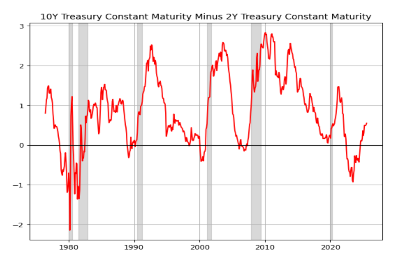
In this chart, we can observe the spread between 10 year and 2 year US Treasuries: the yield curve can be upward sloping or downward sloping and in the latter case the macroeconomic dynamic is called an inversion of the curve.
A change in the spread between the 2-year and 10-year Treasury yields indicates a non-parallel shift in the yield curve, commonly referred to as a curve twist (flattening or steepening process). In a plain vanilla context, where the yield curve slope is positive, flattening can occur: then in an extreme scenario, this can lead to an inverted yield curve, where short-term yields exceed long-term yields, making long-term bonds less profitable on a yield-to-maturity (YTM) basis than short-term ones.
Inversions of the curve are not very common because, after all, they imply that short term rates are higher than long term rates which violates the first rule of finance.
We can also see that every recession (grey areas), from the 1980’s to today has been preceded by an inversion of the curve and that is coherent with the business cycle theory for the yield curve that states that once the yield curve is inverted, this signals that future growth and inflation expectations will contract significantly and that represents a possible recessionary scenario. To be more precise, it is not the inversion of the curve that signals that a recession is coming but it is when the curve steepens up again that signals that a recession is getting closer and so it is important to see how the curve steepens out again because based on the way it does, we can expect different scenarios for the overall economy.
An inverted yield curve can steepen through two processes: bull steepening and bear steepening.
In bull steepening, both short and long-term rates decline, but short rates fall faster, making the curve upward sloping again. This is bullish for bonds as prices rise. This scenario typically occurs when the Fed cuts rates to prevent an economic slowdown or recession. Short rates reflect expectations of lower Fed funds rates, while long rates decline due to reduced growth and inflation expectations—consistent with a recessionary environment. Thus, bull steepening is bullish for bonds but bearish for the economy.
In bear steepening, long-term rates rise faster than short-term rates, eliminating the inversion. This reflects rising growth and inflation expectations, possibly driven by new economic policies, anticipated inflation from tariffs, or concerns over US debt sustainability leading to higher term premiums. This dynamic is bearish for bonds (as prices fall and yields rise), but may signal economic resilience, reducing demand for safe assets like bonds.
Let’s consider how a hedge fund manager can rely on the Treasury yield curve to make a profit from an arbitrage strategy: the spread trade.
A spread trade involves taking two opposite-sign positions on different-maturity bonds, betting on a potential curve twist, usually over a weekly or, rarely, monthly horizon.
Spread Trade: how it works
Spread trade assumes immunization from parallel shifts in the yield curve. If only parallel shifts occurred, spread traders would not face any interest rate risk.
However, as mentioned earlier, the objective is to profit from yield curve twists, while eliminating any exposure to parallel shifts. The only way to achieve this is by neutralizing the portfolio’s duration.
The first step is to calculate the \(\text{DV01}\) (or BPV – Basis Point Value), which represents the theoretical change in price for a one basis point (0.01%) change in yield. The formula is:
\[ \text{DV01} = \text{MD} \times P \times 0.01\% \]Where:
- \(\text{MD}\) is the Modified Duration;
- \(\text{P}\) is the price of the bond.
Then, traders must determine the quantity of each position, by using the Spread Ratio (SR), which is the ratio of the DV01 of the longer-maturity bond to that of the shorter-maturity bond. In numbers:
\[ SR = \frac{\mathrm{DV01}_{\text{long maturity}}}{\mathrm{DV01}_{\text{short maturity}}} \]This means that for each short-term bond bought (sold), the spread trader must sell (buy) SR units of the long-term bond to hedge against parallel shifts.
In the Treasury market, the strategy is implemented using futures. A trader could go long the 2-Year Treasury Note Futures and short the Ultra 10-Year Treasury Note Futures. The strategy works best when using newly issued bonds, which are called OTR (on-the-run) securities.
However, traders must be aware that in the Treasury futures market, the seller of the contract can choose to deliver any eligible security with similar characteristics (delivery option).
The buyer effectively pays the futures price adjusted by a conversion factor (CF), which accounts for differences between deliverable securities. The CF, following the definition of CME Group, represents the estimated decimal price at which \$1 par value of the security would trade if it had a yield to maturity of 6%.
Futures seller will choose the Cheapest-To-Deliver (CTD).
Predicting yield curve twists
Since our goal is to predict the possible movements of the yield curve, the only way to forecast the term spread is by pricing Treasury bonds with constant maturities of 10 and 2 years.
We proceed step by step, using two separate models: one for long-term Treasuries and another for short-term ones.
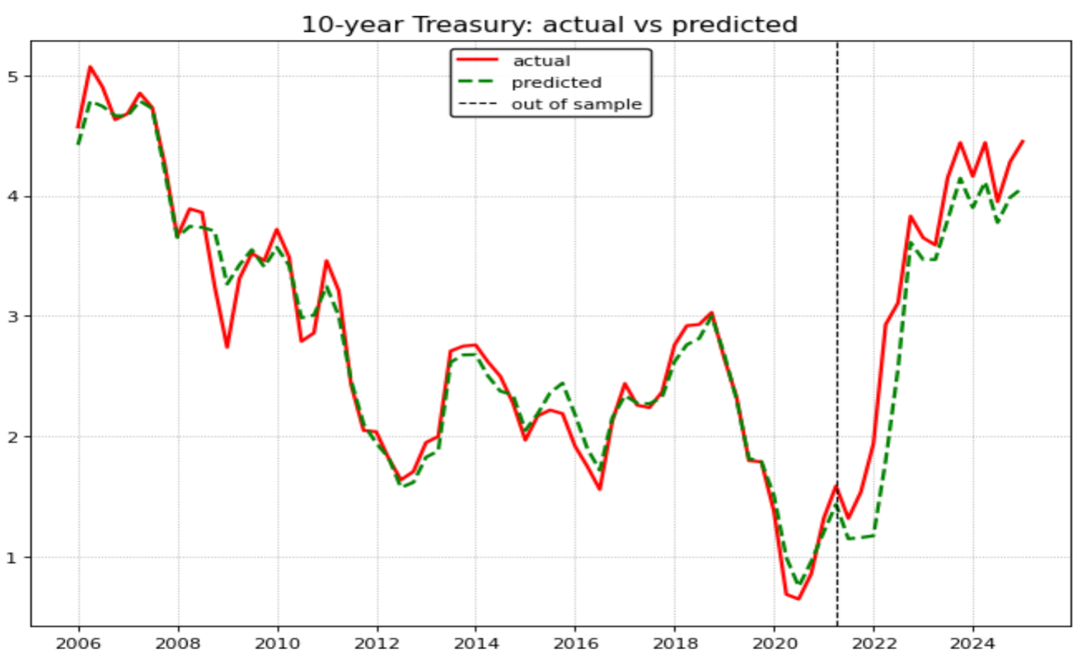
10-year Treasury
For the 10-year Treasury, we refer to Pajusco S. (2025), who states that the bond yield depends on three key financial and macroeconomic variables, consistent with our growth and inflation expectations parameters mentioned before:
- Real GDP growth expectations over the next 10 years, estimated using an ARIMA model;
- 10-year inflation expectations, or Break-Even Inflation (BEI), calculated as the difference between the nominal yield of the 10-year Treasury and the yield of TIPS (Treasury Inflation-Protected Securities);
- Term premium, estimated via the Adrian, Crump, and Moench (ACM) model.
The author constructs an ensemble forecast by averaging the predictions of four models: Ridge Regression, Polynomial Regression, Random Forest Regressor, and XGBoost Regressor.
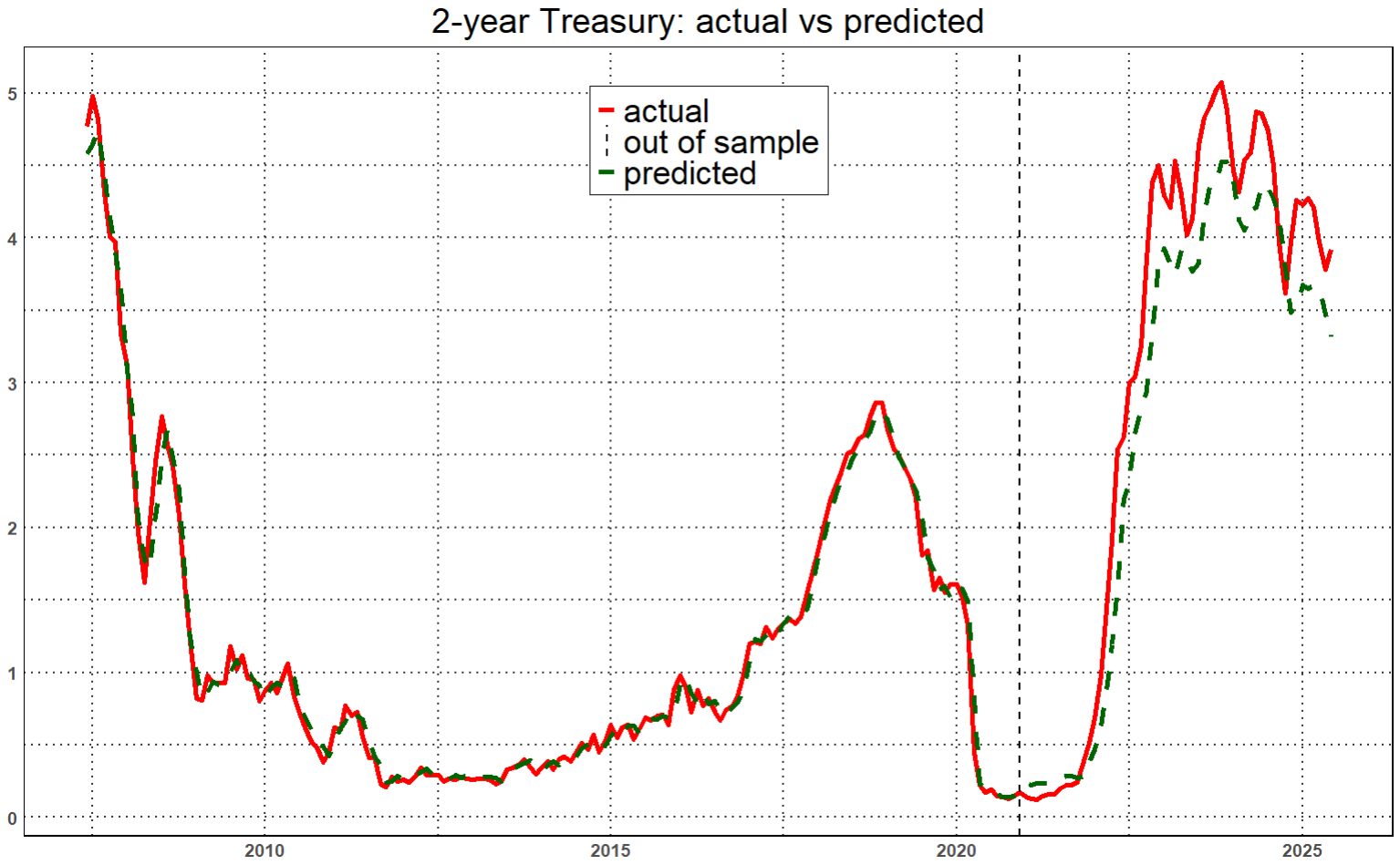
2 Year Treasury
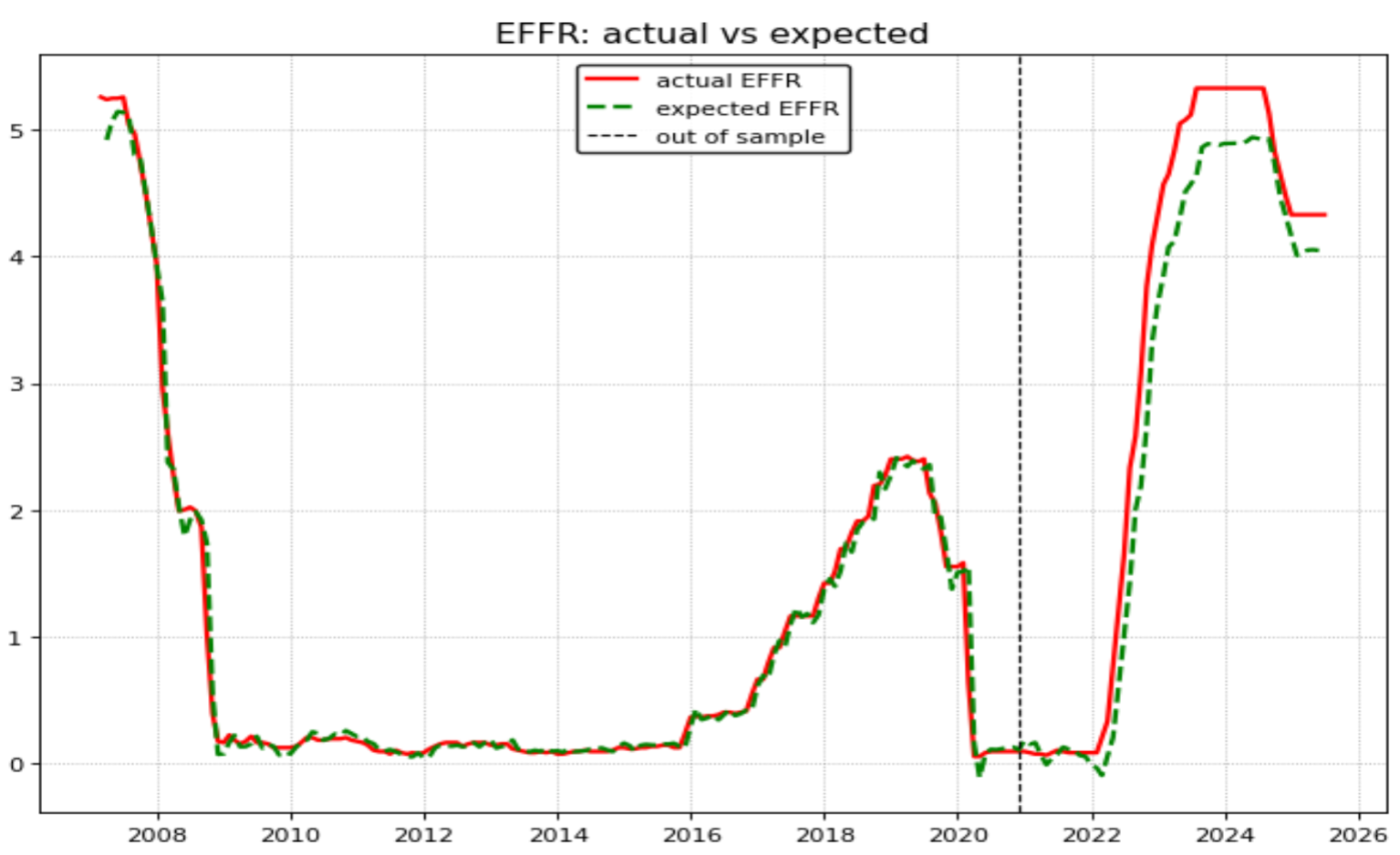
On the other hand, we build a model for the 2-year Treasury yield. To forecast it, we develop an ARIMAX model in which we first attempt to predict the Effective Federal Funds Rate (EFFR) one month ahead, using inflation and labour market indicators, specifically CPI and Nonfarm Payrolls, as explanatory variables to capture monetary policy expectations.
The model performs robustly in-sample, while its out-of-sample accuracy is somewhat weaker. However, this deviation could also suggest that the Fed Chairman has been adopting a more hawkish stance than the fundamentals alone would imply.
Then, we use a Random Forest algorithm to test the 2-year Treasury, utilizing the estimate of the effective Fed fund rate, calculated above, and the DXY percentage changes.
what to do
According to the Jackson Hole speech, a cut in the Fed funds rate is expected. Our ARIMAX model anticipated – by accident – the decrease in the EFFR one year in advance, and the YTD decline in the DXY (\(-13\%\)) could also signal potential demand for short-term Treasuries.
Taking a long position on the 2-year note could therefore mean buying at a moment of relative currency weakness, while also benefiting from a potential reduction in the Fed funds rate, which would increase the value of the bonds purchased.
As far as the long term Treasuries, we expect those rates to go up due to several reasons.
FED is about to cut short term rates even though the most important inflation reports (CPI and PPI) are still higher than the official mandate of 2% per year, like what happened in September 2024 when the FED cut short term rates by 50 bps and the 10 years US Treasuries yield went up significantly.
A higher and higher political pressure on the FED by the Trump administration is pushing for lower rates: these pressures could undermine the independence of the central bank and, ultimately speaking, this could force the central bank to focus more on the maximum employment side of its double mandate, risking a higher than expected long term inflation rate.
The US public debt keeps on growing and despite the DOGE euphoria, the Trump administration has been reluctant to cut the deficits significantly. As a matter fact, the majority of the debt is short term so unless the FED cuts rates dramatically and very quickly, refinancing the debt will happen at a high-rate level and that increases the debt even more. The level of the US debt, as we have seen in the last paper, does not appear to have a significant impact on the level of long term interest rates but at some point (as we are at unprecedented record levels), investors may definitely have to price in a higher credit risk on longer term Treasuries.
By contrast, an alternative view shared by many analysts is that if credit risk were not fully priced, and given that the US gained the upper hand in most of the tariff deals, the U.S. economy could experience stronger real GDP growth than other countries due to reshoring and the foreign investments committed in those agreements. Investors would then adopt a risk-on approach, shifting from safe assets to corporate bonds or stocks, which could lead to a decline in the prices of long-maturity US Treasuries.
So, finally, by taking a long position in the 2-year Treasury while simultaneously shorting the 10-year note—carefully calibrating the positions according to the Spread Ratio (SR) to remain immunized against parallel shifts in the yield curve—investors could potentially exploit relative mispricings between short- and long-term Treasuries.
This arbitrage strategy is designed to take advantage of both anticipated yield curve movements and monetary policy dynamics, effectively offering a “free lunch” opportunity in the current market environment.
Machine Learning Extension
We argued that the profitability of a spread trade, structured as a DV01-neutral long position at the front end of the yield curve and a short position at the long end, depends not on parallel shifts but on twists, specifically the dynamics of steepening and flattening. The short end of the curve was associated with monetary policy expectations, reflected in SOFR and the US Dollar Index, while the long end was linked to growth and inflation expectations, captured by breakeven inflation and term premia. The curve itself, represented by the spread between the 2-year and 10-year Treasury yields, was central to our analysis. In this extension, we developed a machine learning model that formalizes this theoretical framework and evaluates its predictive power.
We employed a bidirectional LSTM (BiLSTM) architecture, designed to capture the sequential and temporal dynamics of yield curve movements. The model was trained on sequences of ninety trading days (roughly a quarter of market data) and tasked with predicting whether the curve would steepen or flatten in the following week. Labels were generated based on weekly changes in the 2s10s spread, with a steepening defined as an increase greater than one basis point, a flattening as a decrease greater than one basis point, and smaller changes ignored to minimize noise. To handle class imbalance, we introduced weighted loss functions.
Two experiments were conducted. In the first, we employed a broader feature set that included yields, breakeven inflation, SOFR, the dollar index, and various rolling measures of spread momentum and volatility. This model achieved a test accuracy of 79 percent. The classification report showed balanced performance across both classes: flattening events were predicted with a precision of 0.77 and a recall of 0.79, while steepening events were predicted with a precision of 0.81 and a recall of 0.79.
Test Accuracy: 0.790

Classification Report:
                precision    recall  f1-score   support

Flattening (0)       0.77      0.79      0.78       144
Steepening (1)       0.81      0.79      0.80       166

      accuracy                           0.79       310
     macro avg       0.79      0.79      0.79       310
  weighted avg       0.79      0.79      0.79       310

Confusion Matrix:
                     Pred Flattening (0)  Pred Steepening (1)
True Flattening (0)                  114                   30
True Steepening (1)                   35                  131
In the second experiment, we restricted the feature set strictly to the variables emphasized in our paper: 2-year and 10-year yields, SOFR, the dollar index, breakeven inflation, and spread dynamics. This restriction resulted in a test accuracy of 75 percent. The classification report revealed a more asymmetric performance. Flattenings were predicted with a precision of 0.67 and a recall of 0.90, while steepenings were identified with a precision of 0.88 but a recall of only 0.62.
Test Accuracy: 0.752

Classification Report:
                precision    recall  f1-score   support

Flattening (0)       0.67      0.90      0.77       144
Steepening (1)       0.88      0.62      0.73       166

      accuracy                           0.75       310
     macro avg       0.78      0.76      0.75       310
  weighted avg       0.78      0.75      0.75       310

Confusion Matrix:
                     Pred Flattening (0)  Pred Steepening (1)
True Flattening (0)                  130                   14
True Steepening (1)                   63                  103
These results highlight a key trade-off. The broader feature set improves overall predictive performance and delivers a more balanced classification of both steepenings and flattenings. The restricted feature set, however, more faithfully reflects the theoretical framework outlined in our paper. Its asymmetric results mirror the intuition that flattenings, often driven by monetary policy tightening, are more readily detectable from short-end indicators, while steepenings, which depend on longer-term growth and inflation expectations, remain harder to anticipate.
There are several limitations to this extension. The lack of direct access to the Adrian–Crump–Moench term premium series, which would have improved the representation of long-end dynamics, forced us to rely on breakeven inflation as a proxy. The definition of labels, based on weekly changes and a fixed one-basis-point threshold, introduces arbitrariness and may fail to capture economically meaningful movements. Furthermore, the model does not incorporate event-driven information such as FOMC meetings or inflation releases, which traders use to anticipate curve shifts. Finally, the BiLSTM framework, while effective in capturing temporal dependencies, may be complemented by alternative architectures, such as temporal convolutional networks or tree-based models, which are well suited for tabular macro-financial data.
Nonetheless, this machine learning extension materially strengthens the paper’s contribution. The results demonstrate that the theoretical pillars of our analysis are sufficiently strong to yield predictive power when formalized in a quantitative model. The restricted-feature model validates the logic of the original framework, while the broader-feature model illustrates the potential of machine learning to refine and enhance predictive accuracy. In this way, the present work bridges the gap between theory and practice, providing both a conceptual and operational foundation for the implementation of spread trades in the US Treasury market.
References
Martellini, L., & Priaulet, P. (2001). Fixed-income Securities: Dynamic Methods for Interest Rate Risk Pricing and Hedging. Wiley.
Boyarchenko, N., Gupta, P., Steele, N., & Yen, J. (2018). Negative Swap Spreads. Federal Reserve Bank of New York.
Pajusco, S. (2025). Predicting the 10-Year US Treasury Yield: An Ensemble Approach Using Macroeconomic Expectations and Term Premia. Riot Investment Research.